Reports
The results of TIMES models are too granular for anyone outside the core modeling team. Modelers normally use Excel workbooks or Powerpoint presentations to share results with clients and stakeholders. Modeling can be more effective if the final consumers of insights can engage with the results directly, not only through the modeling team.
The Reports feature of VO makes this possible.
You can create reporting variables with names that any domain-aware person can understand, like “Electricity Generation” and “Final Energy”, for example. Then you can add an unlimited number of dimensions, like Sector, Fuel, Enduse, Technology, Electricity/CHP, CCS/Non-CCS to disaggregate these reporting variables.
Let’s take Transportation final energy (in a rich model like the JRC_EU-TIMES) as an example: you may want to see energy consumption by scenario, region, fuel, mode, size, and technology. Scenario and region are separate indexes, and fuel can be managed with commodity sets. But we have only process sets to deal with mode, size and technology. The only way is to create three sets of process sets, which have to be viewed separately. The entirely new approach of Reports uses an Excel template to define reporting variables in a very efficient manner, and freely add dimensions based process/commodity names, regions and scenarios. Further, it is possible to include exogenous data in this process, which can be used to include historical energy balances to show historical trends in summary views, and to set up calibration checking views. Population and GDP can be introduced to look at key output per-capita or per unit of GDP.
Note
Examples in this section are based on the JRC_EU-TIMES model. Readers can find more examples in the file LMADefs-EU_TIMES.xlsm.
Reports feature is active in Trial licenses.
Core mechanics of Report creation
The Reports menu can be used to select scenarios, across models and users
Reports are defined in an Excel file (like the Set definitions file)
- There are two basic types of instructions:
Creating variables via combination of attribute, process, commodity, timeslice, and user constraint.
Creating aggregations based on variable, process, commodity and region.
Variables can be created based on process/commodity sets
Tag ~TS_Defs is used to create variables, listed under the column “Name” below. This supports the standard process/commodity filter columns of Veda, along with Attribute, TS (Timeslice) and UC_N. “<Pset>” embedded in the variable name creates a separate variable for each set listed in the PSET_SET column. This works for “<Cset>” and “<CName>” as well.
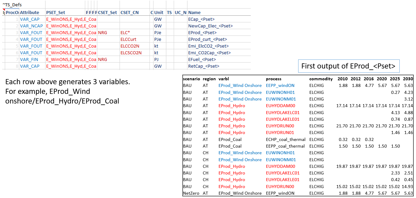
To be embedded in a variable name, the process set should appear in a table ~PSet_Map. This has PSet | Desc | LDesc as columns. Text in the Desc column replaces <PSet> in the variable name. For example, EProd_<PSet> with PSet=ELECOA and Desc=Coal will translate into a variable EProd_Coal. LDesc column is not in use at this time.
Aggregations based on Varbl and Process names
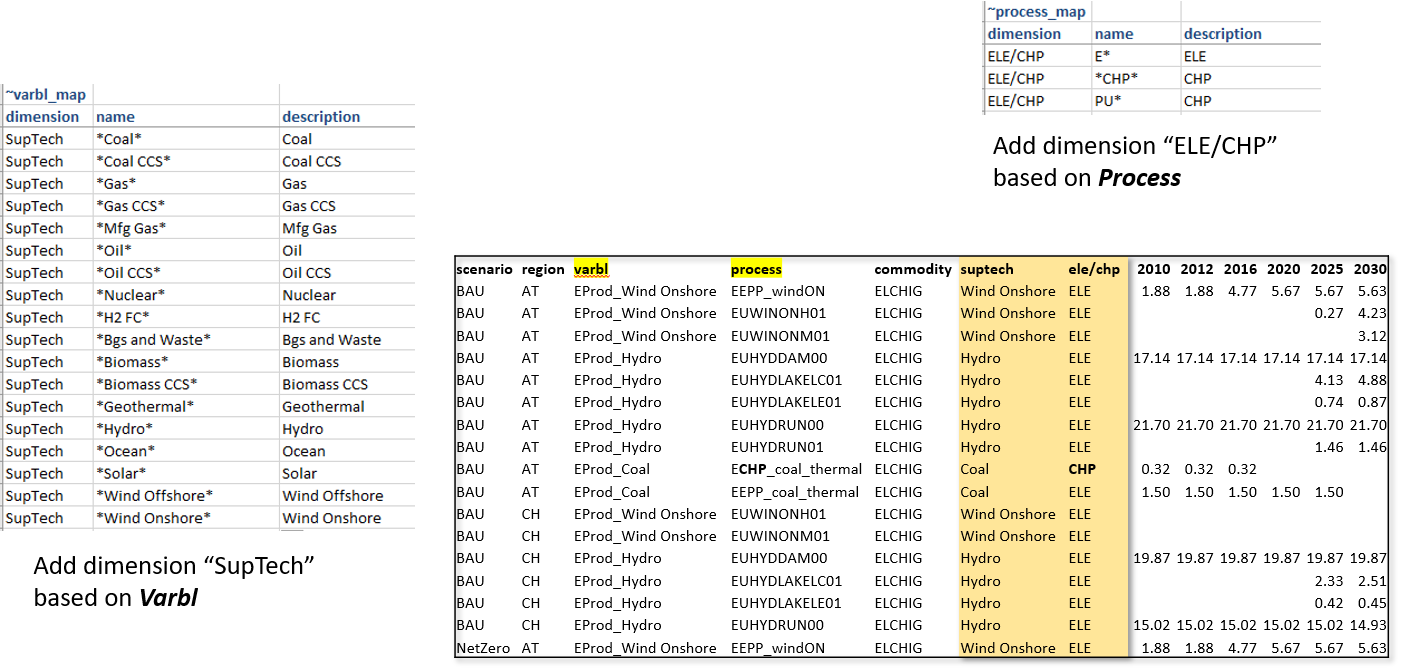
Now we have variables by generation technology, but the technology name is embedded in the variable name, which also has identfiers for the attribute. It would be better to have the technology name in a separate column. Further, one may want to split these variables by ELE/CHP, which could be identified from the process name. Tags ~Varbl_map and ~Process_map make this possible, as shown below.
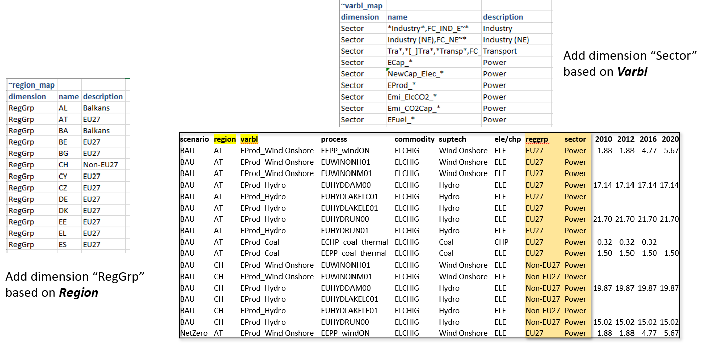
Aggregations based on Varbl and Region names
Region groupings can be created using the ~Region_map tag.
Coarser Variables can be created too
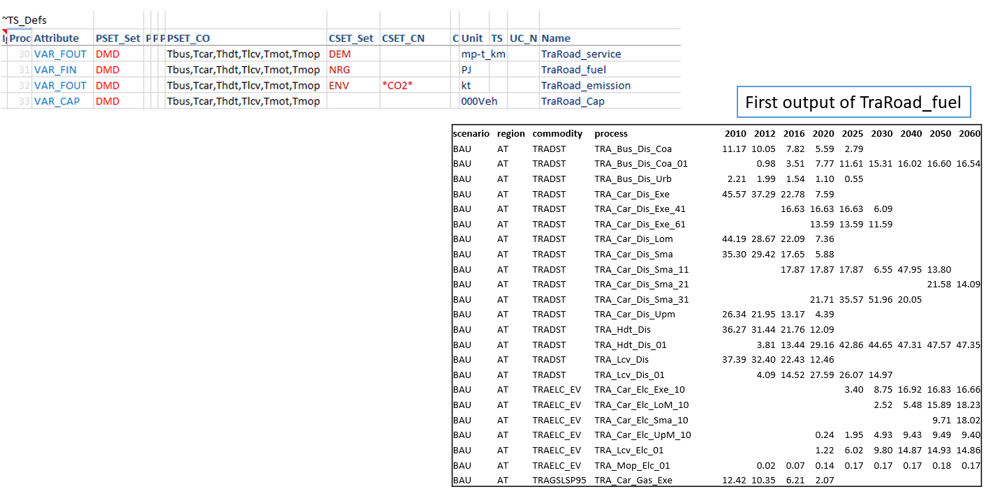
In the first example for creating variables, the technology information was embedded in the variable name (via process set). One can create coarser variables if the naming conventions allow extracting this information directly from process names. We look at the transport sector reporting for this.
Aggregations based on Commodity names
~Commodity_map tag can be used to create commodity aggregations.
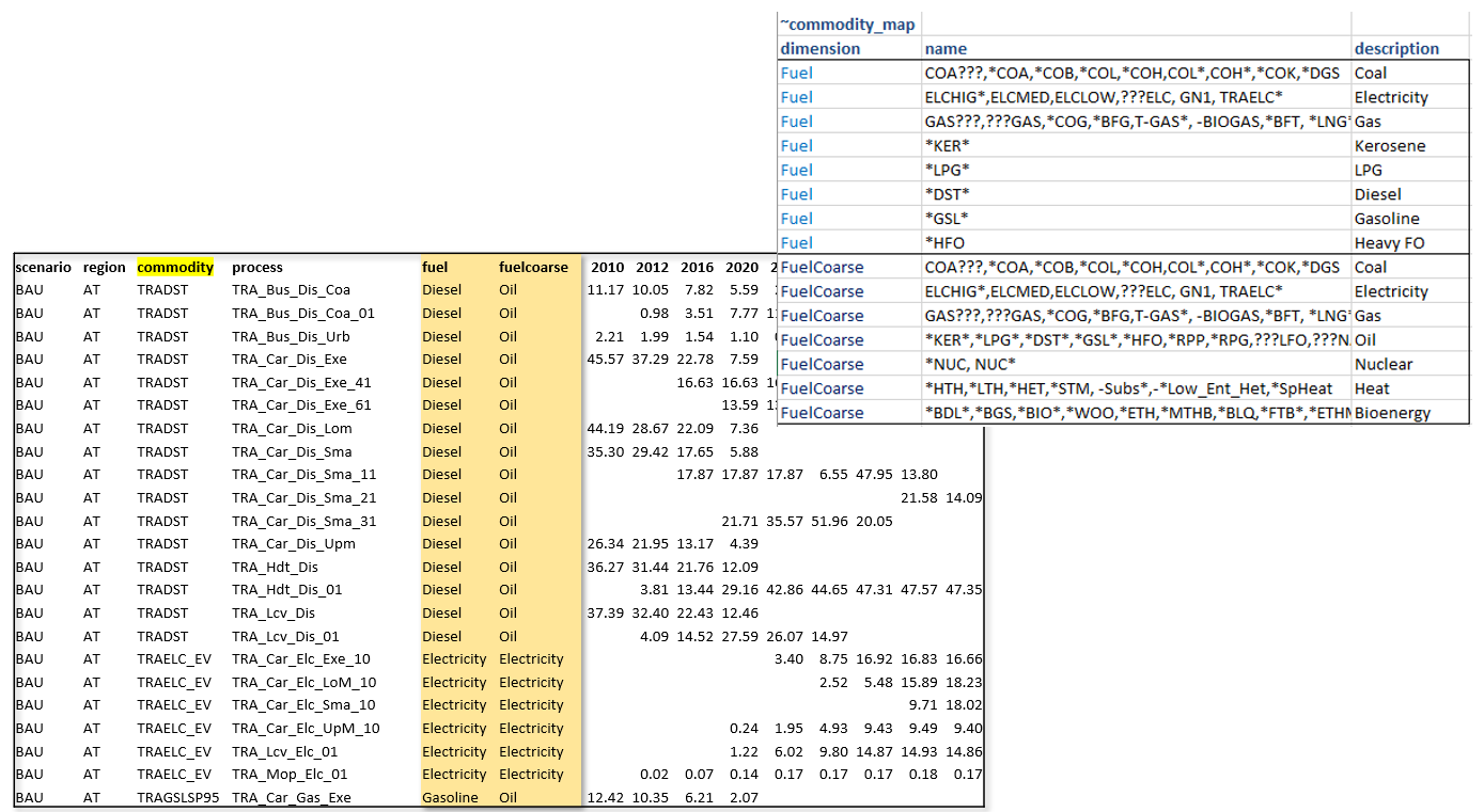
Note
Like in INS tables of Veda, subsequent declarations override the previous ones. For example, you may have several different types of oil, named OILxyz. If you want to track only Oil other, Diesel and Gasoline, then write OIL* | Oil other; OILDST | Diesel; OILGSL | Gasoline, one below the other.
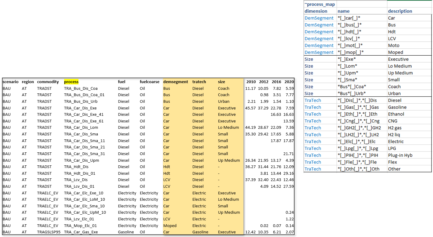
Aggregations based on Process names
Multiple dimensions can be extracted from process names.
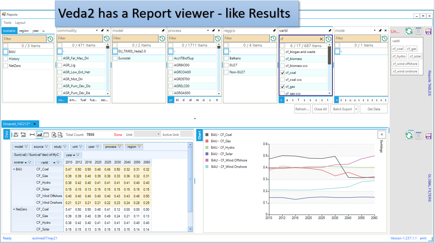
Viewing Reports
Veda2.0 has a basic report viewer, which is sufficient to validate the set up of reports and for simple visualizations. Excel export and CSV dumps are possible, like in Results.
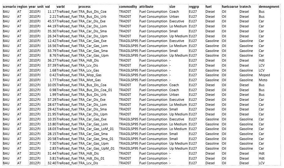
CSV output
It can be consumed in applications like Tableau, Power BI, or LMA
Advanced features
By default process, commodity, and timeslice dimensions are aggregated while generating variables. TS_Defs supports a column “show_me”, where one can indicate dimensions not to be aggregated. Dimensions are indicated by their first characters. “pct” in this column will make process, commodity, and timeslice dimensions survive.
Sankey diagrams: Reports functionality can be used to prepare data for Sankey diagrams. See the report definitions file in JRC_EU-TIMES for one way to do this.
Unit conversion: ~UnitConv tag can be used to convert units. For example, EProd variables can have PJe as the unit, which can be converted to Twh in the report.
- Including exogenous data
Historical trends/calibration check
Producing per/capita and per/GDP metrics
- Special attributes: some ratios are computed based on naming conventions of variables. These are dynamic weighted averages.
Utilization factors
Efficiency (by DEM)
CO2 intensity (by DEM)
Note
It is recommended that one uses “pc” in the “show_me” column when creating new variables, to check the validity of variables and aggregations. Aggregating them makes the reports lighter, so it should be done when possible.
LMA gets a lot more out of Reports
LMA (Last Mile Analytics) is a proprietary web-based data visualization platform, which can be used for many different types of datasets, including results from TIMES models. At this point, LMA is hosted on a server in KanORS office and users have to send VD files to KanORS (along with Report definitions file) to be uploaded. We are in the process of deploying it in the cloud, and eventually users will be able to upload their reports directly from Veda2.0. Access to LMA will not be included in the Advanced license; it will have to be arranged separately.
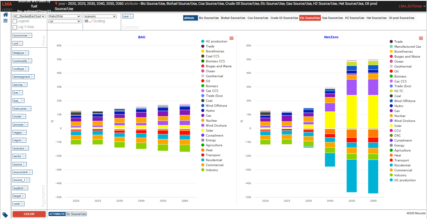
Sources and uses of main energy forms
- See it online select energy form
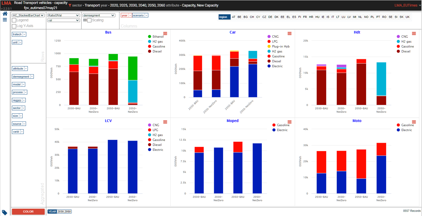
Road transport vehicles
- See it online select region
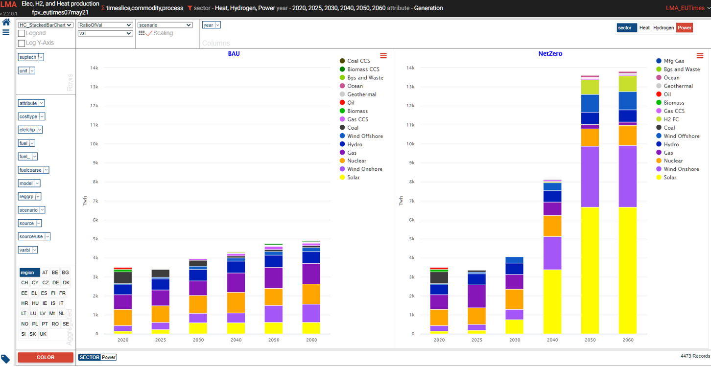
Power generation
- See it online select electricity/hydrogen/heat, and region
Power generation – alternate view
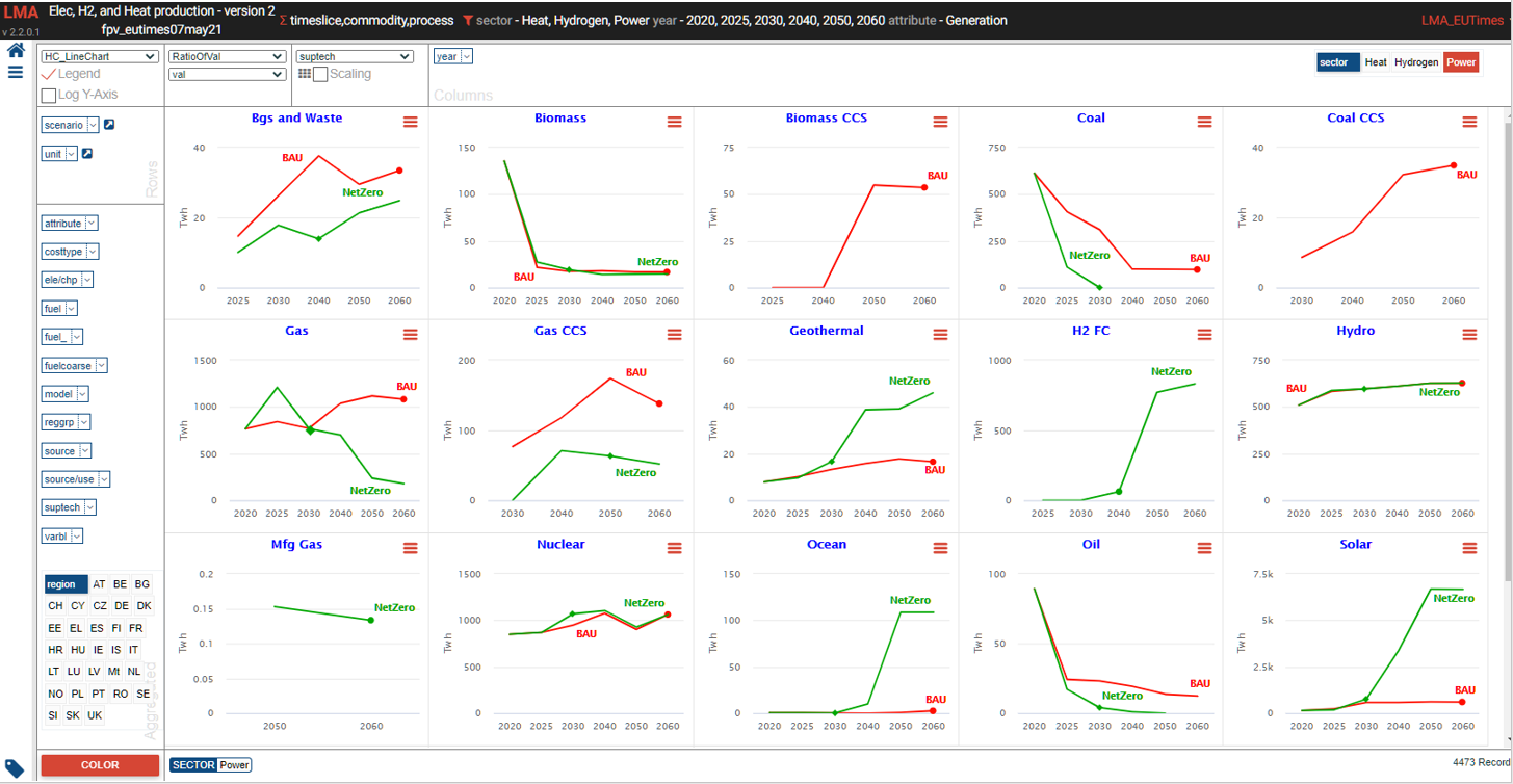
Power generation – alternate view 2
