Reports

Introduction

TIMES model results are often too granular for people outside the core modeling team. Modelers usually share outputs with clients and stakeholders through Excel workbooks or PowerPoint presentations. Modeling becomes more effective when end users can interact with results directly, instead of relying only on the modeling team.

The Reports feature of VO makes this possible.

You can create reporting variables with names that domain users can easily understand, such as “Electricity Generation” and “Final Energy”. You can then add dimensions such as Sector, Fuel, Enduse, Technology, Electricity/CHP, and CCS/Non-CCS to disaggregate those variables.

Take Transportation final energy in a rich model like JRC_EU-TIMES as an example: you may want to view consumption by scenario, region, fuel, mode, size, and technology. Scenario and region are separate indexes, and fuel can be managed with commodity sets. Mode, size, and technology, however, typically require process sets, which are often viewed separately. The Reports approach uses an Excel template to define reporting variables efficiently and add dimensions based on process or commodity names, regions, and scenarios. You can also include exogenous data, such as historical energy balances, for trend analysis and calibration checks. Population and GDP can be included to evaluate outputs per capita or per unit of GDP.

Note

• Examples in this section are based on the JRC_EU-TIMES model. Readers can find more examples in the file LMADefs-EU_TIMES.xlsm.

• Reports feature is active in Trial licenses.

How to use it?

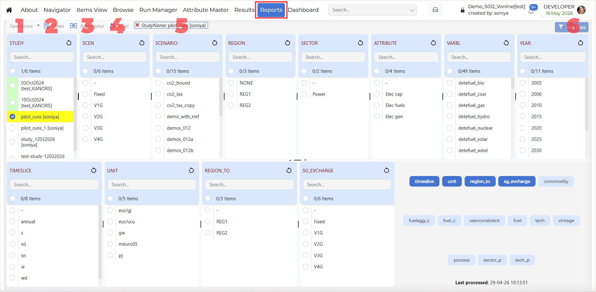
1. Operations

The Operations menu contains actions related to report processing and case management.

• Process Study

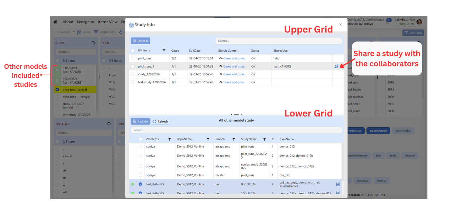
  When Process Study is opened, a Study Info window is shown. This window contains two grids.

  • Upper Grid

    The upper grid contains the studies that belong to the current user or current model.

  • Shared Studies with Collaborators

    To share a study with collaborators from the upper grid, follow these steps

    • To share a study with others, move your mouse pointer over a row in the upper grid. When the user (person) icon appears, click on it to open the Share study with dialog box.

    • Use the search bar to find users or click Select All to choose all available users from the list displayed.

    • Select the desired users.

    • Click Save to share the selected study.

    • Once sharing is complete, the names of the collaborators will appear in the SharedUsers column.

  • Lower Grid

    The lower grid displays studies that have been shared with you from other models-that is, models owned by other users who have chosen to share their studies with you.

  • Including Shared Studies

    To include shared studies from the lower grid, follow these steps

    • Select one or more studies that you want to include.

    • Select one or more studies that you want to include.

    • Click the Include button.

    • The selected studies will be added to your current model for reporting use.

    • You will see a Success message to confirm that the studies were included.

    • Once included

      • These shared studies will appear in the STUDY dimension on the Reports page.

      • Studies that come from another user’s model are highlighted in green for easy identification.

• Delete Cases

  Delete the saved reports in the current model.

2. Views

• The Views option is used to manage saved views.

• Use Views to open the Views window and maintain saved configurations.

• Saved views help users quickly reuse previously defined layouts, filters, and analysis settings without repeating the full setup.

• The Views window contains two main sections:

  1. Views List: shows individual saved views and lets users load, edit, export, delete, or import them.

  2. Views Groups: shows collections of saved views so related analyses can be organized together.

Note

• Use List when you want to work on a specific saved view.

• Use Groups when you want to manage related views as a collection.

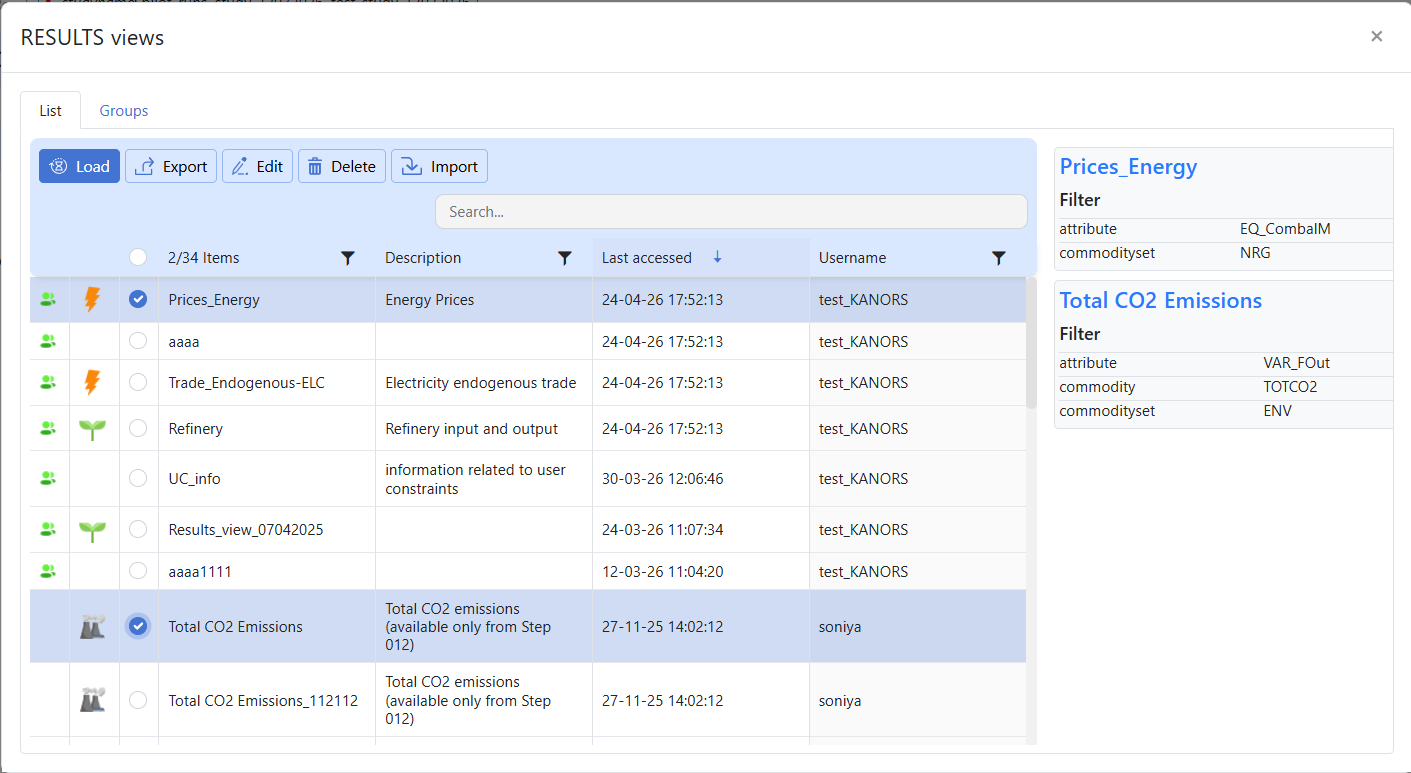
• Views List

  The List tab shows the available saved views. From this section, users can select a saved view and perform actions such as Load, Export, Edit, Delete, and Import.

  • Load

    Use Load to open a previously saved view.

    • Click Views.

    • Stay on the List tab.

    • Select the required saved view.

    • Review the saved filter summary shown in the details panel.

    • Click Load.

  • Export

    Use Export to export a saved view for download.

    • Click Views.

    • Stay on the List tab.

    • Select the required saved view.

    • Click Export.

    • Choose the required download format such as CSV.

    • Confirm the export action.

    • The exported file will be available in the Jobs Dashboard.

  • Edit

    Use Edit to modify an existing saved view.

    • Click Views.

    • Stay on the List tab.

    • Select the required saved view.

    • Click Edit.

    • Change the required filters.

    • Click Update Filters.

    • Confirm the update.

  • Delete

    Use Delete to remove a saved view.

    • Click Views.

    • Stay on the List tab.

    • Select the required saved view.

    • Click Delete.

    • Confirm the deletion, if prompted.

  • Import

    Use Import to bring saved views from another model into the current model.

    • Click Views.

    • Stay on the List tab.

    • Select the required saved view.

    • Click Import.

    • Select the source model.

    • Review the available views.

    • Select the required view or views.

    • If needed, also select the required group of cases.

    • Confirm the import action.

    • Imported views will appear in the Views List with shared icon.

    • Imported groups will appear in the Manage Cases section of the Run Manager, marked with the shared icon.

• Views Groups

  The Groups tab displays saved view groups, where available. This section is used to organize and manage views in grouped form.

Note

• The right-side details panel helps users review saved filter information before loading, editing, exporting, or deleting a view.

• Imported views behave like regular saved views after import.

• Export runs as a background job, and files are downloaded from the Jobs Dashboard.

• Use Edit to update an existing saved view, and Load to open it without making changes.

• A collection of saved views is called a group.

• The Groups tab is used to view and manage groups.

• Groups help users organize related views for easier reuse.

Presenter Views

The Report Presenter Views feature allows controlled sharing of report data.

Sometimes, a user may want to show selected results or analysis to another person, but may not want to give that person access to the complete model, study, or full result dataset.

In such cases, the user can create a Presenter View and share only the required report information.

This helps users share important analysis safely and in a more focused way.

How to use Report Presenter Views?

• Share selected report information with other users

• Present charts, tables, and analysis outputs in a clean format

• Avoid sharing the complete model or study

• Control what information the shared user can view

• Share report data for review, discussion, or presentation

• Provide temporary access to selected report content

Password Protection

• While creating or sharing a Presenter View, the user can set a password.

• This adds an extra layer of security. Only users who have the correct password can open the shared Presenter View.

• Password protection is useful when the shared report contains important or restricted information.

Expiry Date

• The user can also set an expiry date for the Presenter View.

• The expiry date controls how long the shared Presenter View will remain accessible.

• After the expiry date is reached, the shared user will no longer be able to open the Presenter View.

• This helps users share report information for a limited time without keeping access open permanently.

Note

• Report Presenter Views are important because they allow users to share selected information without giving full access to the model or study.

• They provide a controlled and secure way to present report outputs to other users.

• With password protection and expiry date settings, users can decide who can access the Presenter View and for how long.

3. Aggregator

Note

Coming soon. This section will describe the Aggregator feature in Reports.

4. Reset

The Reset option clears the current report selections and removes the applied filters from the page.

5. Global Filters

• The Global Filters default is applied to the latest study.

• When a row in the Results grid is highlighted in yellow, it means that a global filter is applied to that row.

• Press Ctrl key and click on the row to apply the filter to the row.

6. Get Data

The Get Data button retrieves data based on the selected global filters. Use it after selecting the required values in the filter panels.

When a user clicks Get Data Pivot Grid.

Right-click Functionality

The Reports module provides right-click (context menu) capability on selected items in any dimension. This menu offers fast access to key actions relevant to the item you have selected, helping you explore report data more efficiently without navigating away from your main workflow.

Dimension-Specific Options

• Right-click on the selected dimension items to open the context menu. the menu includes the following options:

  • Show Detail – Opens an information dialog with detailed data about the selected item (for example, period - 2015 information or process - COTEELC information).

Core mechanics of Report creation

• The Reports menu can be used to select scenarios, across models and users

• Reports are defined in an Excel file (like the Set definitions file)

• There are two basic types of instructions:

  • Creating variables via combination of attribute, process, commodity, timeslice, and user constraint.

  • Creating aggregations based on variable, process, commodity and region.

Variables can be created based on process/commodity sets

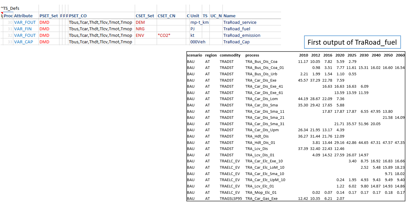
Tag ~TS_Defs is used to create variables, listed under the column “Name” below. This supports the standard process/commodity filter columns of Veda, along with Attribute, TS (Timeslice) and UC_N. “<Pset>” embedded in the variable name creates a separate variable for each set listed in the PSET_SET column. This works for “<Cset>” and “<CName>” as well.

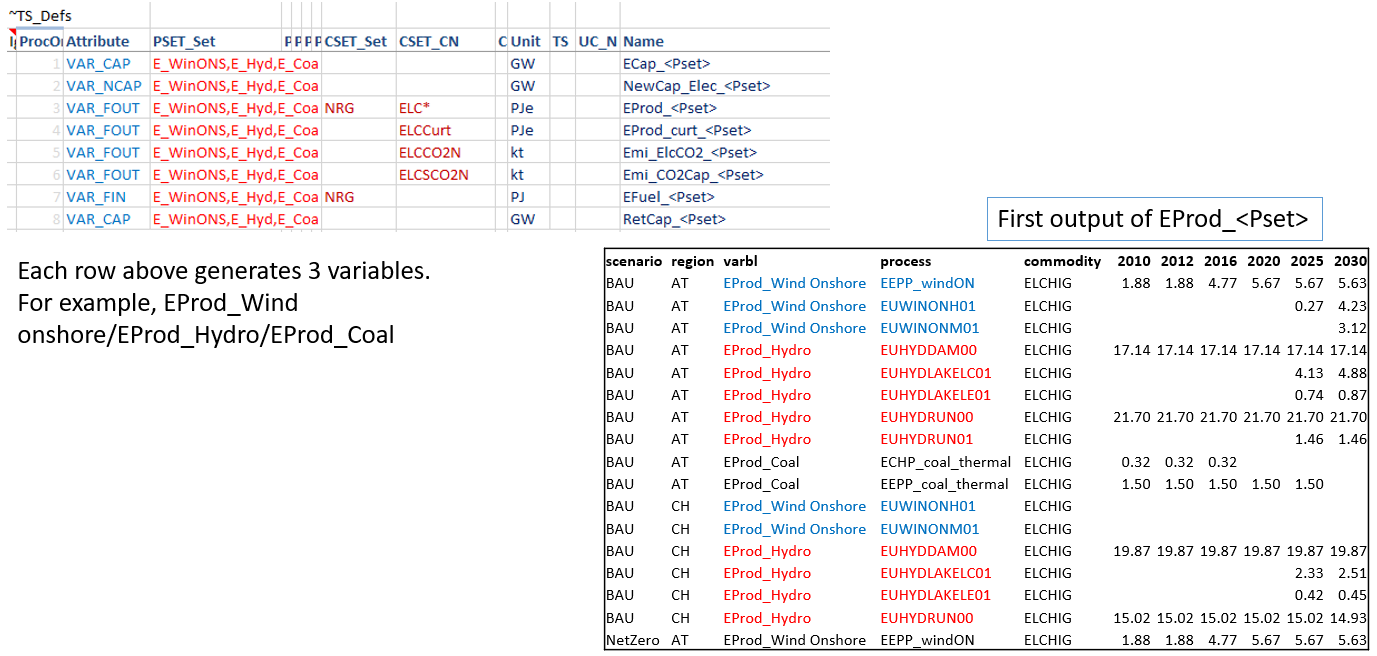
To be embedded in a variable name, the process set should appear in a table ~PSet_Map. This has PSet | Desc | LDesc as columns. Text in the Desc column replaces <PSet> in the variable name. For example, EProd_<PSet> with PSet=ELECOA and Desc=Coal will translate into a variable EProd_Coal. LDesc column is not in use at this time.

Aggregations based on Varbl and Process names

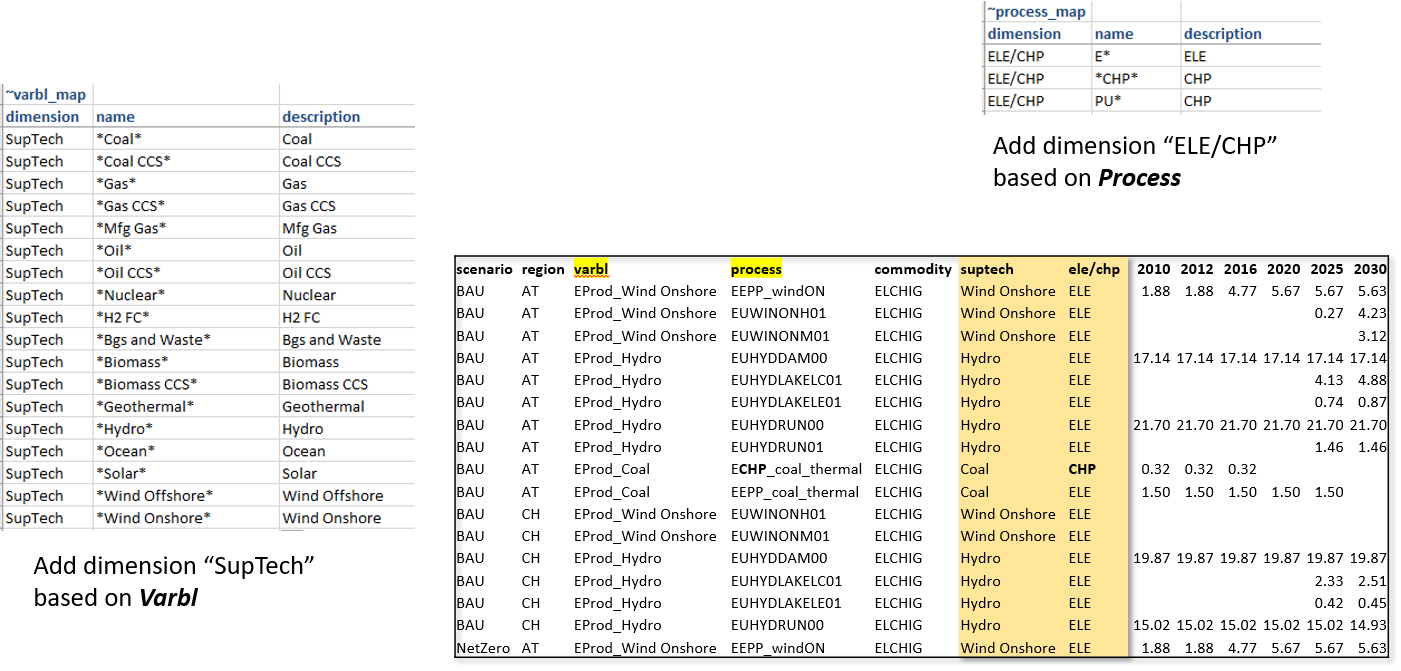
Now we have variables by generation technology, but the technology name is embedded in the variable name, which also has identfiers for the attribute. It would be better to have the technology name in a separate column. Further, one may want to split these variables by ELE/CHP, which could be identified from the process name. Tags ~Varbl_map and ~Process_map make this possible, as shown below.

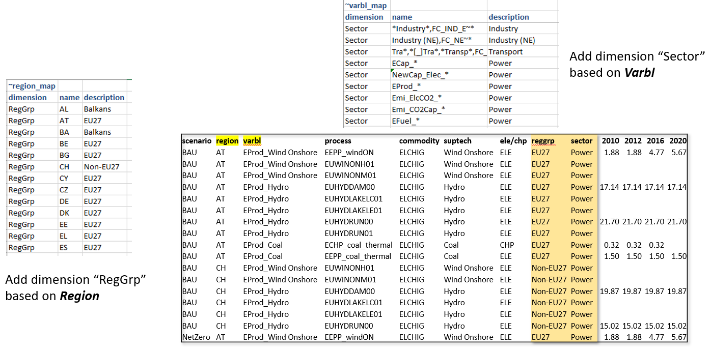
Aggregations based on Varbl and Region names

Region groupings can be created using the ~Region_map tag.

Coarser Variables can be created too

In the first example for creating variables, the technology information was embedded in the variable name (via process set). One can create coarser variables if the naming conventions allow extracting this information directly from process names. We look at the transport sector reporting for this.

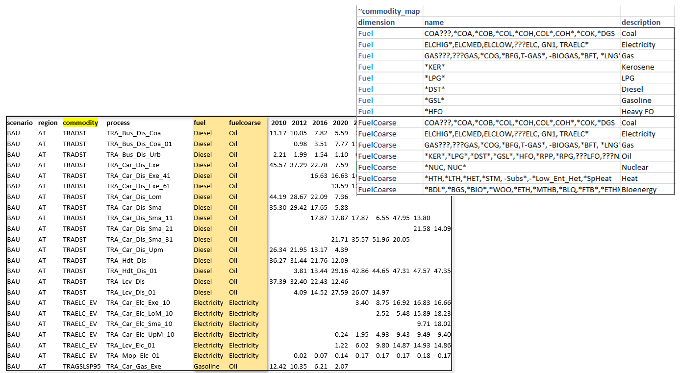
Aggregations based on Commodity names

~Commodity_map tag can be used to create commodity aggregations.

Note

Like in INS tables of Veda, subsequent declarations override the previous ones. For example, you may have several different types of oil, named OILxyz. If you want to track only Oil other, Diesel and Gasoline, then write OIL* | Oil other; OILDST | Diesel; OILGSL | Gasoline, one below the other.

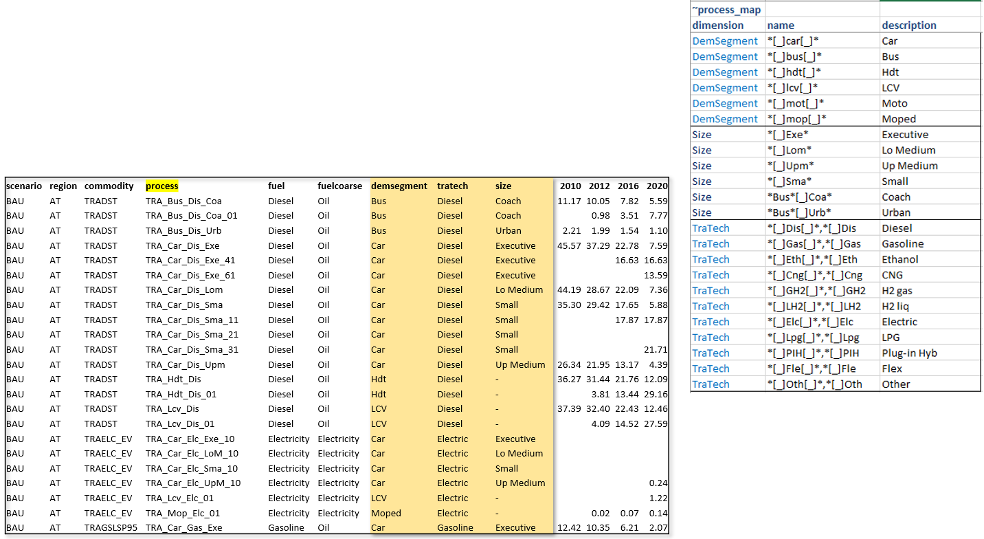
Aggregations based on Process names

Multiple dimensions can be extracted from process names.

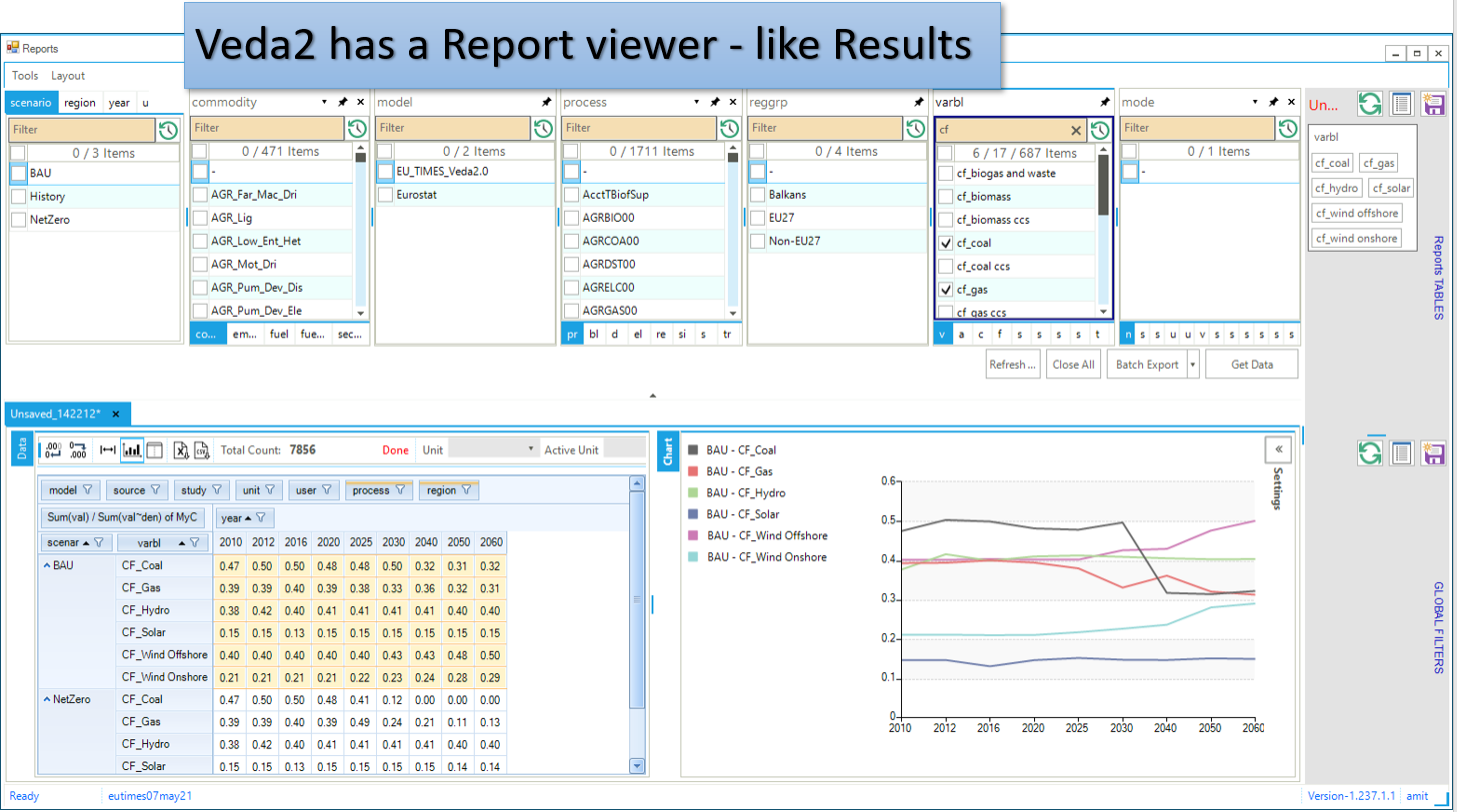
Viewing Reports

Veda2.0 has a basic report viewer, which is sufficient to validate the set up of reports and for simple visualizations. Excel export and CSV dumps are possible, like in Results.

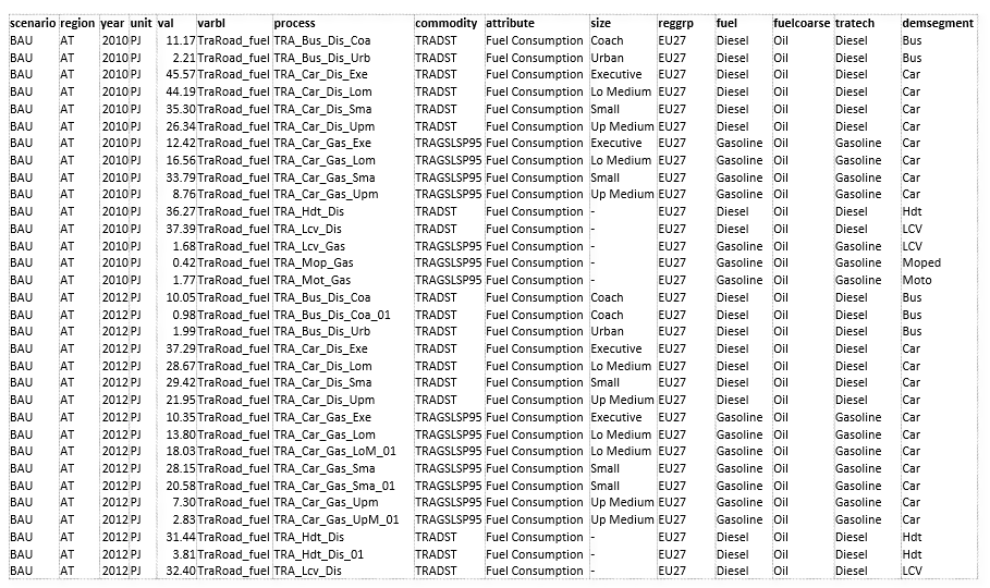
CSV output

It can be consumed in applications like Tableau, Power BI, or LMA

Advanced features

• By default process, commodity, and timeslice dimensions are aggregated while generating variables. TS_Defs supports a column “show_me”, where one can indicate dimensions not to be aggregated. Dimensions are indicated by their first characters. “pct” in this column will make process, commodity, and timeslice dimensions survive.

• Sankey diagrams: Reports functionality can be used to prepare data for Sankey diagrams. See the report definitions file in JRC_EU-TIMES for one way to do this.

• Unit conversion: ~UnitConv tag can be used to convert units. For example, EProd variables can have PJe as the unit, which can be converted to Twh in the report.

• Including exogenous data

  • Historical trends/calibration check

  • Producing per/capita and per/GDP metrics

• Special attributes: some ratios are computed based on naming conventions of variables. These are dynamic weighted averages.

  • Utilization factors

  • Efficiency (by DEM)

  • CO2 intensity (by DEM)

Note

It is recommended that one uses “pc” in the “show_me” column when creating new variables, to check the validity of variables and aggregations. Aggregating them makes the reports lighter, so it should be done when possible.

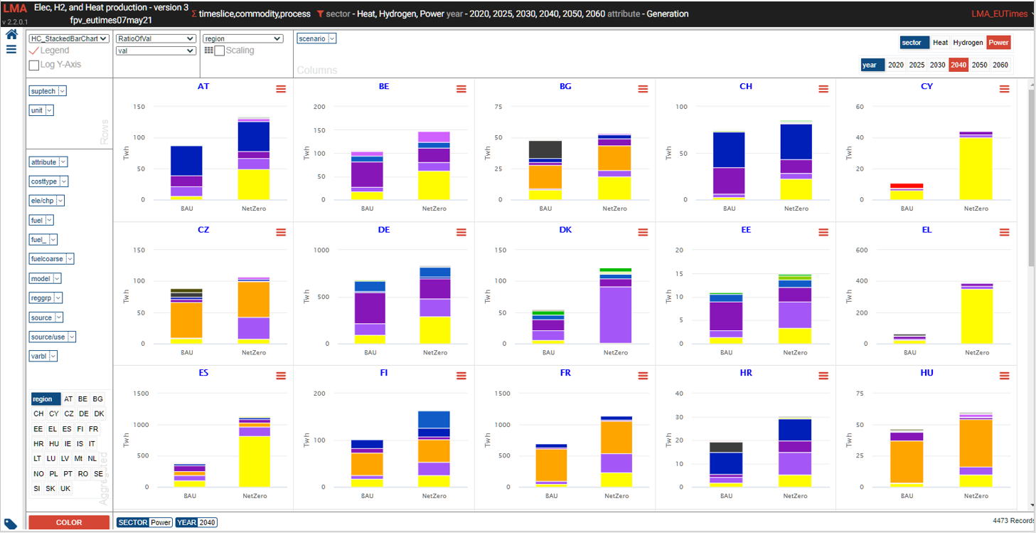
LMA gets a lot more out of Reports

LMA (Last Mile Analytics) is a proprietary web-based data visualization platform, which can be used for many different types of datasets, including results from TIMES models. At this point, LMA is hosted on a server in KanORS office and users have to send VD files to KanORS (along with Report definitions file) to be uploaded. We are in the process of deploying it in the cloud, and eventually users will be able to upload their reports directly from Veda2.0. Access to LMA will not be included in the Advanced license; it will have to be arranged separately.

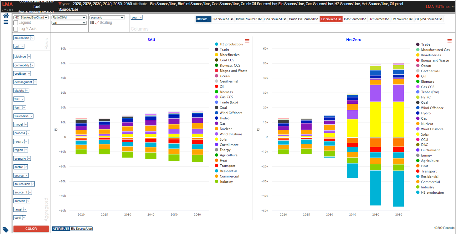
Sources and uses of main energy forms

• See it online select energy form

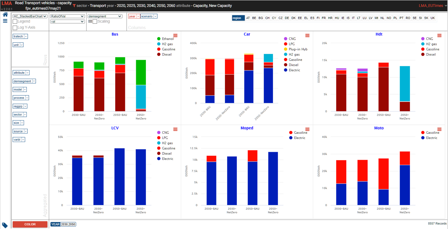
Road transport vehicles

• See it online select region

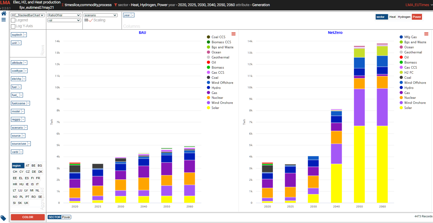
Power generation

• See it online select electricity/hydrogen/heat, and region

Power generation – alternate view

• See it online

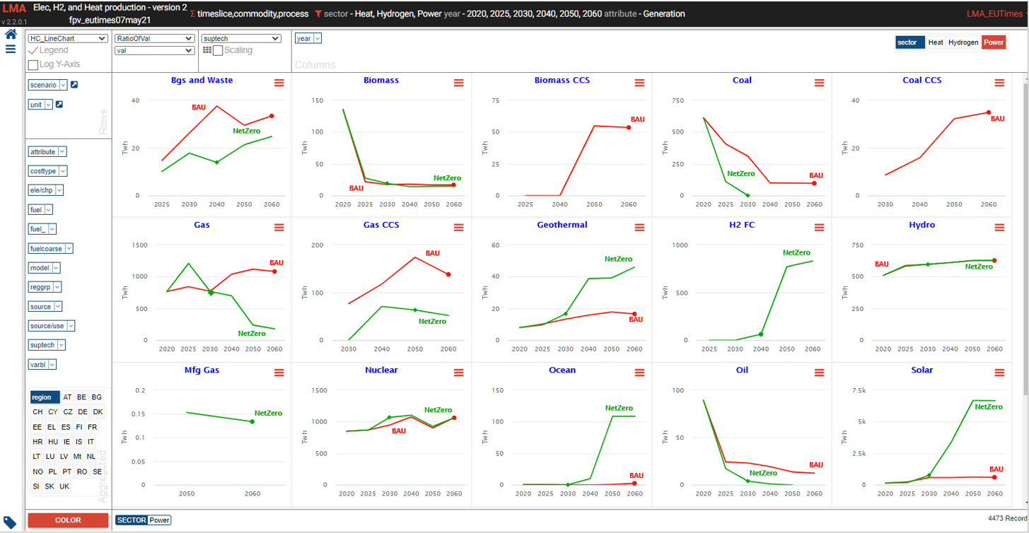
Power generation – alternate view 2

• See it online